Histograms

Students look at a bar chart and a histogram, compare/contrast them, and make observations about what they have in common and how they are different. Then they learn a more formal explanation of histograms.

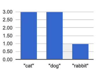The display on the right side of that page is a Bar chart.

The display on the right side is called a histogram.

To build a histogram, we start by sorting all of the numbers in our column from smallest to largest, marking our x-axis from the smallest value (or a bit below) to the largest value (or a bit above) and dividing into equally-sized or bins (also known as intervals). For example, if our values ranged from 3 to 53 we might mark our x-axis from 0 to 60 and divide it into bins of width 10. If they range from 22 to 41 we might mark our x-axis from 20 to 45 and divide it into bins of width 5. Once we have our bins, we put each value in our dataset into the bin where it belongs, and then count how many values fall in each bin. This count determines the height of the bars on our y-axis.

In the histogram we just made, we see that the data is clustered at the right-hand side of the histogram: most people in this sample have close to a full set of teeth, with some people missing a few more than others. But apparently there are five people with almost no teeth at all! These are very unusual, and they show up as a small bar far to the left of the cluster. Extreme data points like this are called outliers.

Note that intervals on this display include the left endpoint but not the right. If we included the right endpoint and someone had 0 teeth, we’d have to add on a bar from -5 to 0, which would be awfully strange!

Review: How are histograms and bar charts different?

Students make histograms from the animals-dataset, and explore different bin sizes.

The size of the bins matters a lot! Bins that are too small will hide the shape of the data by breaking it into too many short bars. Bins that are too large will hide the shape by squeezing the data into just a few tall bars. In this exercise, the bins were provided for you. But how do you choose a good bin-size?

Suppose we want to know how long it takes for animals from the shelter to be adopted.

Optionally, provide students with Choosing the Right Bin Size, a handout with space to respond to the guided questions below.

If someone asked what was a typical adoption time, we could say: “Almost all of the animals were adopted in 10 weeks or less, but a couple of animals took an unusually long time to be adopted — even more than 20 or 30 weeks!” It would have been hard to give this summary by reading through the table, but the histogram makes it easy to see!

Students apply what they have learned about histograms to their chosen dataset. They will add two items to their Data Exploration Project Slide Template: (1) at least two histograms and (2) any interesting questions that emerge. To learn more about the sequence and scope of the Datatset Exploration Project, visit Project: Dataset Exploration. For teachers with time and interest, Project: Create a Research Project is an extension of the Dataset Exploration, where students select a single question to investigate via data analysis.

Let’s review what we have learned about making and interpreting histograms.

Let’s connect what we know about histograms to your chosen dataset.

Confirm that all students have created and understand how to interpret their histograms. Once you are confident that all students have made adequate progress, invite them to access their Data Exploration Project Slide Template from Google Drive.

Share your findings with the class!

Did you discover anything surprising or interesting about your dataset?

What questions did the bar and pie charts inspire raise?

Did other students make any discoveries that were surprising or interesting to you? (For instance: Did everyone find outliers? Was there more or less similarity than expected?)