Suppose you’re visiting a new city, and you want to go out for a great meal. Someone suggests a really expensive restaurant, and assures you it’s the best in town. How do you know if you’re being ripped off? You now have significant experience asking questions about data sets: You know how to take measures of center, and how to visualize both categorical and quantitative data. Let’s use this experience to find out if the expensive restaurants are really worth the money. First, we’ll start with out data set: a table containing information about the restaurants in town.
name
price
rating
"Family Diner"
13.21
4.5
"Geoff’s Sandwiches"
10.23
4.1
"Best Burger"
6.52
2.9
"Riverside Grille"
19.56
4.9
"Jackie’s BBQ"
5.57
2.3
"La Taqueria"
9.72
4
"Bebop Bar"
7.2
3.3
"Spike’s"
6.98
3.8
"Fred’s Shake Shack"
5.25
3.5
Here the name column is the name of the restaurant, the price contains the average price of an entree at the restaurant, and the rating column contains the average star rating given by customers.
Are more expensive restaurants generally better than cheaper ones?
Turn to page Page 20. Take two minutes and write down what you think.
Encourage students to discuss openly before writing.
What tables do you see defined here? What other definitions do you see?
What is the highest average price for a restaurant?
Use Pyret to define ratings-list and prices-list as two lists representing the rating and price columns of the restaurants table.
Use Pyret to calculate the mean star rating (out of 5 stars) of the restaurants.
Use Pyret to visualize the average prices of restaurants with a histogram.
Use Pyret to create a scatter plot showing the average prices and average review ratings of all the restaurants.
According to this plot, do you think expensive restaurants have higher ratings?
Students should extract the price column, and use the max function. Then, look through the table to find the row with that price, and look at the entry in the name column.
Students should extract the rating column and use the mean function.
Students should extract the price column, and use the histogram function over the list.
Students should create a scatterplot, using what they learned in previous lessons.
Students won’t know how to answer this yet, and that’s ok!
In the last question, we are asking about the relationship between two columns of quantitative data: price and rating. As the price increases, what happens to the rating? Does it increase as well?
To answer this question, we will return to the very first chart you learned about in this class: scatter plots. A scatter plot is a chart that plots every pair of numbers in 2 columns. By extracting the two columns from restaurants, we can create a series to plot:
Click Run, and show the scatterplot for prices-vs-ratings-plot
There are 9 points on our restaurant scatter plot: one for each restaurant in the table. Each dot’s placement depends on the price and rating values of a particular restaurant. For example, look at the restaurant "Riverside Grille". Riverside Grille has an average price of 19.56, so it will appear to the far right of the chart. Riverside Grille has an average rating of 4.9, so it will appear towards the top of the chart.
In Pyret, open the scatter plot that shows the relationship between prices and ratings.
Which dot represents the restaurant "Family Diner"?
If there were a 10th restaurant with an average price of $11, and a rating of 3.5, where should that dot be?
Do more expensive restaurants in this chart tend to have higher ratings or lower ones? What about the chart makes you think so?
If there were another restaurant with an average price of $16, what is our best guess for what its rating might be, based on this scatter plot?
This last question motivates the idea of prediction: using the general shape of the data to estimate values.
For practice, try making scatter plots for each of the following relationships:
The fat vs. calories-from-fat columns of nutrition.
The gdp vs median-life-expectancy columns of countries
The population vs media-life-expectancy columns of countries
Scatter plots are a simple way to visualize the relationship between two columns of quantitative data. In this scatter plot, we can see a general trend that restaurants with higher price tend to be rated higher. This particular example might seem intuitive, but it’s a lot easier to search for relationships in data using a visualization than a table by itself.
Turn to Page 21 in your workbook and complete the exercise practicing creating scatter plots.
Seeing Correlations
Overview
Learning Objectives
Evidence Statements
Product Outcomes
Materials
Preparation
Seeing Correlations
(Time 25 minutes)
We noticed that higher-rated restaurants tended to be better-reviewed. This relationship is called a positive correlation, because an increase in one measurement (price) tended to result in an increase in the other (rating). What do you think it would mean if we saw a negative correlation?
Scatter plots are useful when searching for a relationship between two columns of quantitative data. Often, if we find a relationship, we can use that relationship to make predictions. For example, we predicted that a restaurant with a price of $16 would have a rating somewhere between 4 and 5. A prediction summarizes the relationship within our data cloud, for example "for every $4 in price, a restaurant’s rating tends to be a full point higher".
Students’ predictions may differ from between [4, 5]. If so, guide them towards why this range is intuitive.
Correlations help us make predictions, but not every prediction is right! We might predict that a cheap restaurant won’t be as good as a fancy one, but sometimes the local diner is actually better than fancy bistro! Height is positively correlated with being good at basketball - but that doesn’t mean a taller player is always better!
Brainstorm three positive correlations you see in the world around you, as well as three negative ones. Can you think of exceptions where the correlation does not hold?
But how do measure a correlation? Can something be "more positively" or "more negatively" correlated than another? Are some correlations stronger or weaker than others?
We can represent a positive correlation by drawing a line on a scatter plot, representing the prediction.
This line is the graph of a predictor function. A predictor is a function that takes in a value for one variable, and returns an estimate of a different variable, based on all the other points in the cloud. In our example, we can predict the rating of a restaurant, based on its price.
For each point, use the linear predictor to estimate the answer.
What’s the expected rating of a restaurant with an average price of $12?
What’s the expected price of a restaurant with an average rating of 3?
What’s the expected rating of a restaurant with a price of $8?
Emphasize that the predictor isn’t always exactly correct, but if the data shows a direct correlation, then the predictor will be pretty close. This makes it very useful for problems where it is hard to gather lots of data.
We can be reasonably confident in our predictor function, because it looks like it matches our data set. But what would it look like if we had a predictor that didn’t match? Let’s take a look at a different predictor function.
This line would give close predictions for restaurants with average prices around $4 or $6, but for higher prices it’s completely wrong. What makes this predictor so bad?
It is bad because it doesn’t match the shape of the data.
Complete Page 22 in your workbook, by grading different predictor functions on how well they match scatter plots (on a scale of 0="worst fit" to 1="best fit").
Some of these scatter plots showed positive correlations. Others showed negative correlations: where if one variable increases, the other decreases, and vice versa. There are also examples where the line doesn’t appear to have much value as a predictor; in these examples we say there is no correlation.
Linear Regression
Overview
Learning Objectives
Evidence Statements
Product Outcomes
Materials
Preparation
Linear Regression
(Time 35 minutes)
This leaves us with two questions:
How do we make a prediction from a scatterplot? In other words, "how do we know where to draw that line?"
How do we measure the accuracy of our prediction? In other words, "how well does that line fit?"
Data scientists use statistics to build a model of a data set. This model takes into account a lot of different measures (including some of the ones you already know), and tries to identify patterns and relationships within the data. We can build a model of our own in Pyret, and grab a predictor function from it:
linear-regression is a function that takes 2 lists as arguments, and returns a function of Type Number -> Number. This function is our predictor, representing the line that best fits the data. We define this function to be the identifier rating-predictor, and we can use it just like any other function.
Type rating-predictor(0) into the Interactions Area. What is the output? What happens with rating-predictor(20)? What is the contract for rating-predictor?
You can learn more about how a predictor is created by watching this video.
If you want to teach students the algorithm for linear regression (calculating ordinary least squares), now is a good time to do it!
Once we have the function series, we know how to plot it - we used draw-plot back in Unit 1! Use Pyret to plot this function, and the scatter-plot. Ideally, we’d like to plot these on top of one another, and we can do this using the draw-plots function. It works much the way draw-plot does, but instead of one series it takes in a list of series (List<Series>) as its Domain.
Create statistical models and predictor functions for each of the following relationships, then plot the predictor function on top of the scatterplots you created earlier:
The fat vs. calories-from-fat columns of nutrition.
The total gdp vs median-life-expectancy columns of countries
The total population vs median-life-expectancy columns of countries
Make sure to adjust the bounds to see all of the data on each one. Also, use the appropriate axis labels.
It may be helpful for students to copy and paste the example code that constructs a scatter plot for these examples, and modify it.
Are there any correlations in this data? If so, what are they?
Strong correlation between fat and calories from fat
Almost no correlation between GDP and life expectancy - Note: sharp-eyed students will point out that this is total GDP, not per-per-capita, so we don’t expect much correlation!
Almost no correlation between Population and life expectancy
In your workbook activity, you gave predictors "grades" for how well they performed. Data scientists use r-squared values to grade predictors in real life.
Type r-squared(prices-list, ratings-list, rating-predictor) into the Interactions Area.
This is a number on the same scale [0, 1] that tell us "how much of the variation in the scatterplot is explained by this function". In other words, it’s a measure for how well the line fits. A perfect score of 1.0 means that 100% of the variability in the data is explained by the function, and that our predictor is perfect. For the price vs ratings, the predictor score is ~0.71, which is fairly accurate. The contract for r-squared is:
Determine the r-squared values for each of the 3 models you created previously, and interpret them. Do they show a strong correlation? A weak correlation? No correlation at all?
What does it mean a data point is above the predictor line?
What does it mean a data point is below the predictor line?
If you only have two datapoints, why will the r-squared value always be 1.0?
Have your students examine the r-squared values for the life expectancy models. Population size has virtually no correlation, but GDP has roughly 30%! Is this surprising to the students? Did they expect it to be stronger or weaker? How can they explain the result?
Optional: teach your students how r-squared values are calculated.
Complete Page 23 in your workbook, by writing your own definitions for predictor function, and vocab{r-squared}.
Closing
Overview
Learning Objectives
Evidence Statements
Product Outcomes
Materials
Preparation
Closing
(Time 10 minutes)
Turn to Page 20, and take two minutes to write down your findings. In your answer, include the fact that you used linear regression to come up with a predictor. Bonus points for explaining what the r-squared value tells about that prediction!
Open your Final Project document, and answer question 8. What correlations do you think are lurking in your dataset?
Suppose you could divide your data up, perhaps by the kind of restaurant, or by the neighborhood where the restaurant is located. If you ran a linear regression on a per-neighborhood basis, do you think you would find a stronger correlation? Perhaps a different correlation? If your dataset includes both men and women, you might want to re-run the analysis on the genders separately. To do any of this analysis, you’ll need to learn how to manipulate tables, so you can sort them, break them apart, or add new columns. The next three units will show you how to do just that.

 There are 9 points on our restaurant scatter plot: one for each restaurant in the table. Each dot’s placement depends on the price and rating values of a particular restaurant. For example, look at the restaurant "Riverside Grille". Riverside Grille has an average price of 19.56, so it will appear to the far right of the chart. Riverside Grille has an average rating of 4.9, so it will appear towards the top of the chart.
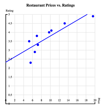 We can represent a positive correlation by drawing a line on a scatter plot, representing the prediction.
 We can be reasonably confident in our predictor function, because it looks like it matches our data set. But what would it look like if we had a predictor that didn’t match? Let’s take a look at a different predictor function.